Simulate stochastic choices

author: steeve laquitaine

This tutorial simulates the stochastic choices generated by a cardinal Bayesian model.

Setup

# go to the project's root path
import os
os.chdir("..")

# import dependencies
from bsfit.nodes.models.bayes import CardinalBayes
from bsfit.nodes.dataEng import (
    simulate_task_conditions,
)
import pandas as pd
%load_ext autoreload
%autoreload 2

The autoreload extension is already loaded. To reload it, use:
  %reload_ext autoreload

Set the parameters

# set the parameters
PRIOR_SHAPE = "vonMisesPrior"
PRIOR_MODE = 225
OBJ_FUN = "maxLLH"
READOUT = "map"
PRIOR_NOISE = [80, 40]      # e.g., prior's std
STIM_NOISE = [0.33, 0.66, 1.0]
SIM_P = {
    "k_llh": [2.7, 10.7, 33],
    "k_prior": [2.7, 33],
    "k_card": [2000],
    "prior_tail": [0],
    "p_rand": [0],
    "k_m": [2000],
}
GRANULARITY = "trial"
CENTERING = True
N_REPEATS=5

Simulate task conditions (design matrix)

# simulate task conditions
conditions = simulate_task_conditions(
    stim_noise=STIM_NOISE,
    prior_mode=PRIOR_MODE,
    prior_noise=PRIOR_NOISE,
    prior_shape=PRIOR_SHAPE,
)

The task conditions are shown below:

conditions

	stim_mean	stim_std	prior_mode	prior_std	prior_shape
0	5	0.33	225	80	vonMisesPrior
1	10	0.33	225	80	vonMisesPrior
2	15	0.33	225	80	vonMisesPrior
3	20	0.33	225	80	vonMisesPrior
4	25	0.33	225	80	vonMisesPrior
...	...	...	...	...	...
67	340	1.00	225	40	vonMisesPrior
68	345	1.00	225	40	vonMisesPrior
69	350	1.00	225	40	vonMisesPrior
70	355	1.00	225	40	vonMisesPrior
71	360	1.00	225	40	vonMisesPrior

432 rows × 5 columns

Simulate stochastic choices

# instantiate the model
model = CardinalBayes(
    initial_params=SIM_P,
    prior_shape=PRIOR_SHAPE,
    prior_mode=PRIOR_MODE,
    readout=READOUT
    )

# simulate stochastic choice predictions
output = model.simulate(
    dataset=conditions,
    granularity=GRANULARITY,
    centering=CENTERING,
    n_repeats=N_REPEATS
)

Running simulation ...

-logl:nan, aic:nan, kl:[ 2.7 10.7 33. ], kp:[ 2.7 33. ], kc:[2000.], pt:0.00, pr:0.00, km:2000.00

The simulated dataset is shown below.

output["dataset"]

	stim_mean	stim_std	prior_mode	prior_std	prior_shape	estimate
0	5	0.33	225	80.0	vonMisesPrior	55
1	5	0.33	225	80.0	vonMisesPrior	23
2	5	0.33	225	80.0	vonMisesPrior	238
3	5	0.33	225	80.0	vonMisesPrior	317
4	5	0.33	225	80.0	vonMisesPrior	237
...	...	...	...	...	...	...
2155	360	1.00	225	40.0	vonMisesPrior	71
2156	360	1.00	225	40.0	vonMisesPrior	67
2157	360	1.00	225	40.0	vonMisesPrior	208
2158	360	1.00	225	40.0	vonMisesPrior	193
2159	360	1.00	225	40.0	vonMisesPrior	290

2160 rows × 6 columns

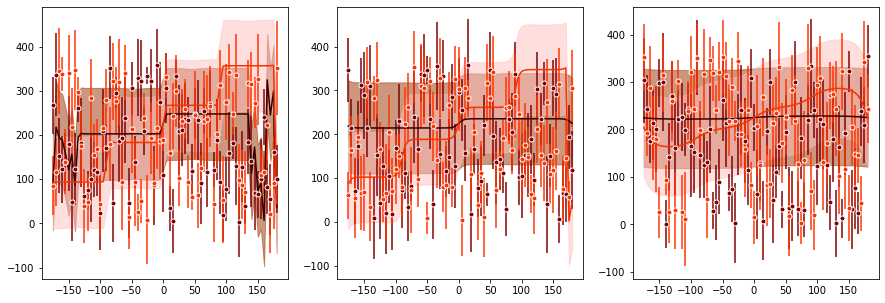
Calculate estimate choice statistics

# simulate predictions
from matplotlib import pyplot as plt
plt.figure(figsize=(15,5))
model = model.simulate(
    dataset=output["dataset"],
    sim_p=SIM_P,
    granularity="mean",
    centering=CENTERING,
)

Running simulation ...

Calculating predictions ...

-logl:12717.25, aic:25452.49, kl:[ 2.7 10.7 33. ], kp:[ 2.7 33. ], kc:[2000.], pt:0.00, pr:0.00, km:2000.00

A preview of the unique 431 combinations of task conditions (prior noise, stimulus noise, stimulus feature) is shown below:

pd.DataFrame(output["conditions"]).head()

	0	1	2
0	80.0	0.33	5.0
1	80.0	0.33	10.0
2	80.0	0.33	15.0
3	80.0	0.33	20.0
4	80.0	0.33	25.0

Model’s estimate generative probability density: the probability that the model generates each estimate is shown below, with the estimates ranging from 0 to 359 in the rows and each unique 431 combinations (prior noise, stimulus noise, stimulus feature) in the columns:

pd.DataFrame(output["PestimateGivenModel"]).head()

	0	1	2	3	4	5	6	7	8	9	...	422	423	424	425	426	427	428	429	430	431
0	0.004032	0.003639	0.00324	0.002972	0.002842	0.002795	0.002781	0.002778	0.002778	0.002778	...	0.00275	0.00275	0.002749	0.002749	0.002747	0.002746	0.002745	0.002744	0.002744	0.002744
1	0.004032	0.003639	0.00324	0.002972	0.002842	0.002795	0.002781	0.002778	0.002778	0.002778	...	0.00275	0.00275	0.002749	0.002749	0.002747	0.002746	0.002745	0.002744	0.002744	0.002744
2	0.004032	0.003639	0.00324	0.002972	0.002842	0.002795	0.002781	0.002778	0.002778	0.002778	...	0.00275	0.00275	0.002749	0.002749	0.002747	0.002746	0.002745	0.002744	0.002744	0.002744
3	0.004032	0.003639	0.00324	0.002972	0.002842	0.002795	0.002781	0.002778	0.002778	0.002778	...	0.00275	0.00275	0.002749	0.002749	0.002747	0.002746	0.002745	0.002744	0.002744	0.002744
4	0.004032	0.003639	0.00324	0.002972	0.002842	0.002795	0.002781	0.002778	0.002778	0.002778	...	0.00275	0.00275	0.002749	0.002749	0.002747	0.002746	0.002745	0.002744	0.002744	0.002744

5 rows × 432 columns

Here is a list of the attributes generated by the simulation:

list(output.keys())

['PestimateGivenModel',
 'map',
 'conditions',
 'prediction_mean',
 'prediction_std',
 'dataset']

Tutorial complete !